There are two important factors relative to lead times in your supply chain. One, of course, is to know the actual lead times that you are experiencing relative to various SKU-Locations (or, SKULs). The other key factor is the variability of the lead time.
In virtually all ERP (enterprise resource planning) systems, the databases capture all of the data necessary to understand these factors.
How to begin
You begin by simply capturing the correlated data between supply orders (e.g., purchase orders, work orders, transfer orders) and their related fulfillment transactions (e.g., receipts of goods, work order production transactions).
From these data, it should be relatively easy to have a tool (such as Microsoft Excel or Transact-SQL [T-SQL]) calculate the actual number of days between the supply order and the supply fulfillment.
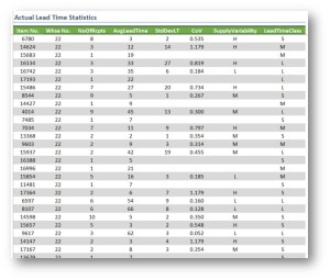
In the accompanying figure, we see these data summarized. We have the columns Item Number, Warehouse Number, Number of Receipts, and Average Lead Time.
Lead-Time classes
One valuable extrapolation from these data is to classify the lead times. A good start is to simply break the lead times into three broad categories—short lead times, medium lead times and long lead times. Precisely where the line of demarcation falls between these three classes of lead times will depend upon a number of factors related to a firm's industry and its situation in the supply chain.
A simple to identify starting point for breaking out these classes into short, medium and long is to sort the entire range of data by Average Lead Time and then call the bottom third the short lead-time section; the middle third the medium lead-time, and the remaining the long lead-time SKULs. In our example, the lower limit of the medium lead-time range is nine days, and the upper limit for the medium range is 21 days.
Supply variability
The next critical factor is a measure for variability in supply. To get to this metric, we use two calculations: the first is a calculation of the standard deviation in the lead-time days. This is done easily enough using standard functions in T-SQL or Excel. Standard deviation is an absolute measure of how much each data point in a record set departs from the mean (or average).
The second calculation is what is frequently referenced as coefficient of variability (CoV). This metric compares the ratio of the standard deviation to the average (Standard Deviation / Average). The higher the CoV, the greater the variability in the data set. This is important to know because a nine-day standard deviation in a 70-day average lead time would constitute only a 0.129 CoV; whereas, a nine-day standard deviation against a 10-day average lead time would constitute a CoV of 0.900.
Having calculated the CoV, it makes a good deal of sense to break your SKULs into manageable groups based on CoV ranges. Low, medium and high variability groups are indicated in the figure in the Supply Variability column.
NOTE: Since standard deviation cannot be calculated where only a single receipt of goods is recorded, the standard deviation LT, CoV, and Supply Variability columns are all empty in the figure.
Next steps
Having calculated and taken note of these factors, these factors can now be used in a system designed to determine proper target inventory levels. Typically, SKULs with longer lead times would use smaller adjustment factors, and SKULs with shorter lead times would employ larger adjustment factors when calculating the size of each SKUL's buffer size.
If you would like more information on how to do these calculations from your database (like an example T-SQL query) and recommendations about how to calculate inventory buffer sizes using these factors, please feel free to contact me.


